
Sankey diagrams are used to testify flow between two or more categories, where the width of each individual element is proportional to the period charge per unit. These nautical chart types are available in Power BI, but are non natively available in Excel. However, today I desire to evidence you lot that it is possible to create Sankey diagrams in Excel with the right mix of elementary techniques.
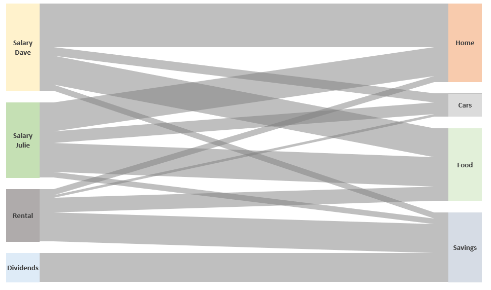
While Sankey diagrams are often used to show energy flow through a process, beingness a finance guy, I've decided to evidence cashflow. The uncomplicated Sankey diagram above shows four income streams and how that cash and so flows into expenditure or savings.
Download the example file
I recommend you download the example file for this post. And so yous'll exist able to work along with examples and see the solution in activity, plus the file volition exist useful for futurity reference.
![]()
Download the file: 0050 Sankey diagrams in Excel.xlsx
Watch the video
This web log post will exist slightly dissimilar from others; rather than show you how to do each step, I volition demonstrate the overall approach. There are additional details covered in the YouTube video.
Lookout man the video on YouTube.
The hush-hush
While I should expect to reveal the hugger-mugger until the end of the post, I call up it will help to explicate how it all fits together if I reveal it upfront.
Here is the underground: the Sankey diagram yous see in the example file is not one chart, far from information technology. There are actually 21 charts all stacked on tiptop of each other.
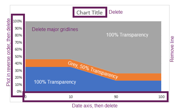
The following epitome shows the 21 private charts that could make up a Sankey diagram.
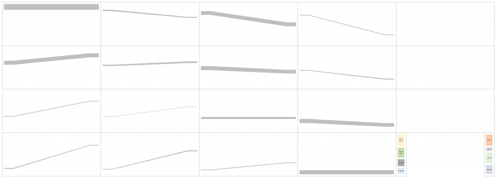
By setting the backgrounds to be fully transparent, and the shaded lines as partially transparent; overlaying the charts on top of each other creates the Sankey effect. The pillars at each end are 100% stacked cavalcade charts, which are also overlaid on top.
Now that I've revealed how elementary this hush-hush is, let'south wait at each stage in a bit more than detail. Then you will be able to create your ain Sankey diagram templates.
Initial data
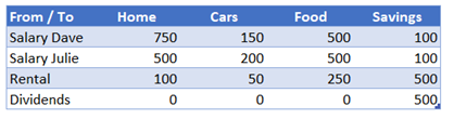
Our initial data is a 2-dimensional table. The rows are the start point for our Sankey diagram, while the columns are the endpoint. The value at the intersection of these is the flow rate.
Inside the template, we also have a named range called Bare. The value in here represents the spacing to be applied between each category.![]()
Formula Magic with Dynamic Arrays
 Of all the features available in Excel dynamic arrays provide the about ability for the smallest time investment. Yet most Excel users do not even know what they are.
Have you always faced these spreadsheet scenarios?
- How can Iuse VLOOKUP to render all the matching items, not just the get-go?
- How can Isort my information using a formula, so I don't have to go along clicking the sort button?
- How can I quicklycreate unique lists of items to utilize with my SUMIFS calculation?
- How can Istop copying down formulas every fourth dimension my source data changes.
- How can I build aPivotTable-like report, but using formulas so I don't have to click refresh always again.
Well, I'm hither to give y'all some good news. with dynamic arrays, all these tin be accomplished easily 🙂

Interim calculation tables
To create the Sankey effect from our initial information, we demand to create interim calculations.
- SankeyLines table
- SankeyStartPillar table
- SankeyEndPillar tabular array
- Spacing named range
Let'due south wait at each in turn.
SankeyLines table
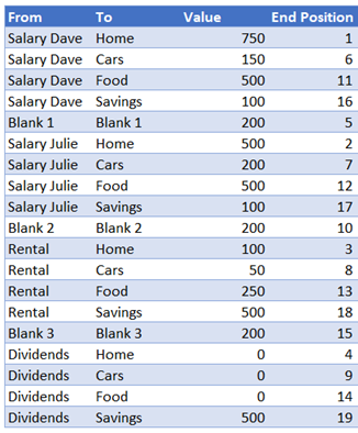
From the source data, we create a table with a row for each possible combination of rows and columns. This table is called SankeyLines table in the case file. Each row category is separated by an additional line which creates the blank spaces we see in the charts.
Our initial SankeyLines table needs to contain the following base data:
Value
The formula in the Value column is:
=IF(LEFT([@From],5)="Bare",Bare, INDEX(SankeyData,MATCH([@From],SankeyData[From / To],0), MATCH([@To],SankeyData[#Headers],0)))
This formula retrieves either:
- Value from the source table
- Value of the Blank named range (where it is a row used for spacing between categories).
End Position
The End Position cavalcade determines the social club of the lines at the end of the Sankey diagram. Where ane is finishes at the acme, 2 is the second item from the top, etc.
SankeyLines table additional data points
To create the information for the 100% stacked surface area chart, nosotros need to summate some additional data points:
- Space to a higher place the shaded Sankey line
- Value of the shaded Sankey line
- Space below the shaded Sankey line
Our SankeyLines table needs to expand with the following calculations.
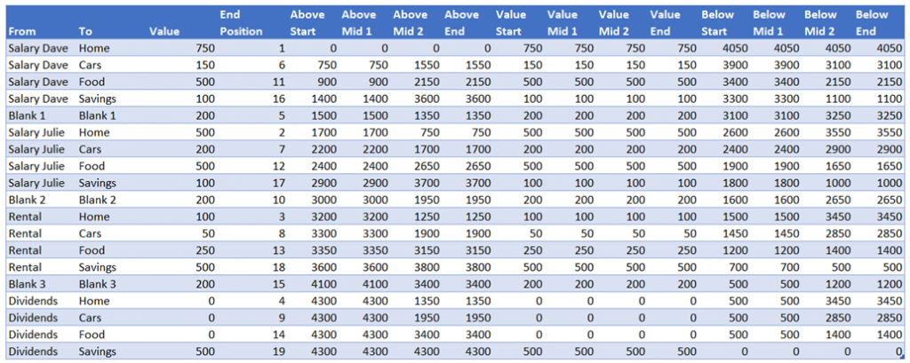
The formulas in each column are as follows:
Above Start
=SUM(SankeyLines[[#Headers],[Value]]:[@Value])-[@Value]
This calculates the amount of space required above the Sankey line at the outset point.
Above Mid 1
=[@[Above Start]]
This is sent to equal the Above Start cavalcade.
Higher up Mid ii
=[@[Above Terminate]]
This is fix to equal the Above End column (see below)
To a higher place End
=SUM([Value])-SUMIFS([Value],[Terminate Position],">="&[@[Cease Position]])
This calculates the corporeality of space required higher up the Sankey line at the end signal.
Value Start, Value Mid 1, Value Mid 2, Value Terminate
=[@Value]
The tiptop of the shaded Sankey line never changes. Therefore, we tin fix the value of all 4 columns to equal the Value column.
Below Start, Below Mid 1, Below Mid two, Below Finish
The columns calculate the amount of space required below the shaded Sankey line. Each calculation is constructed the aforementioned way. It takes the SUM([Value]) then takes away the value from the equivalent First, Mid 1, Mid 2 or End columns.
Below Kickoff:
=SUM([Value])-[@[To a higher place Showtime]]-[@[Value Outset]]
Beneath Mid ane:
=SUM([Value])-[@[To a higher place Mid 1]]-[@[Value Mid one]]
Below Mid 2:
=SUM([Value])-[@[Higher up Mid 2]]-[@[Value Mid 2]]
Below Stop:
=SUM([Value])-[@[In a higher place End]]-[@[Value Terminate]]
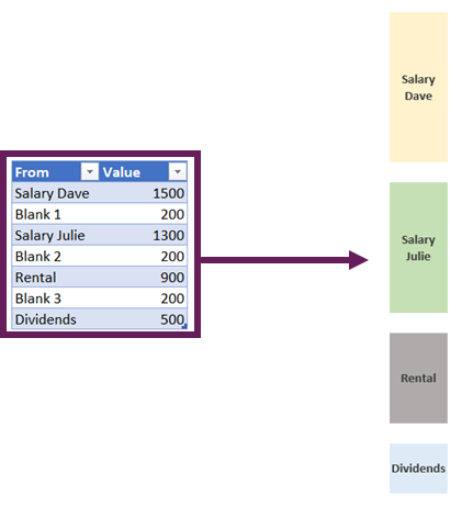
SankeyStartPillars table
The SankeyStartPillar tabular array is reasonably easy to sympathize. Information technology merely needs each row category from the source data listed with a "Blank" particular in between.
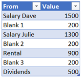
The formula for the Value column is:
=SUMIFS(SankeyLines[Value],SankeyLines[From],[@From])
End pillars
The SankeyEndPillar table is like to the SankeyStartPillar table. It just needs each column category from the source data listed with a "Blank" item in between.
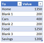
The formula for the Value is:
=SUMIFS(SankeyLines[Value],SankeyLines[To],[@To])
Spacing named range
The final office of the interim calculations is a named range called Spacing. This is used as the Category (horizontal) Centrality for the chart. It determines at what point the slope of the chart starts and finishes.
![]()
Nautical chart layering
Once all the interim calculations are gear up, the chart creation can begin.
Create the individual shaded Sankey lines
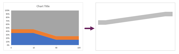
Each row of the SankeyLines table needs to exist a separate 100% stacked area nautical chart with 3 data serial:
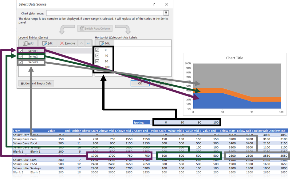
Once the chart has the correct serial data, it so all comes down to formatting.
After all the formatting has been completed the chart will become a single grey line.
If the row in the SankeyLines table starts with "Blank", then technically it can be deleted, however for completeness, I prefer to go on it in that location, but set it to No Fill. Information technology means that if I always demand to utilize it, I can just modify the make full color and it can exist used as a standard shaded Sankey line.
Once all the shaded Sankey lines have been created, they can be overlaid on top of each other.

Create the Sankey pillars
Nigh of the hard piece of work has now been completed. We just need to create 2 100% stacked column charts—one for the showtime pillar and i for the end pillar.
The pillars are set to be formatted as follows:
- Plot series in reverse order
- Your preferred fill colors
- Set the "Blank" sections with No Fill up
- Add together data labels to the relevant points.
Afterward all of that, we overly the pillars on top of our nautical chart. Finally, our Sankey diagram is complete.
Decision
That'due south it. Individually there is goose egg too difficult with any of the techniques involved. But they demand to exist combined in the right mode to create the Sankey outcome. Initially, this takes quite a long time to create, but once fix-up, it can be used over and over with different categories. It'due south definitely the case of invest the fourth dimension once, to create a template large enough and so and reuse information technology.

Go our Free VBA eBook of the 30 nearly useful Excel VBA macros.
Automate Excel so that y'all can save time and stop doing the jobs a trained monkey could do.
Past entering your email address you agree to receive emails from Excel Off The Grid. We'll respect your privacy and you can unsubscribe at any time.
Don't forget:
If you've found this postal service useful, or if you have a better arroyo, so please go out a comment below.
Do you need help adapting this to your needs?
I'm guessing the examples in this postal service didn't exactly meet your state of affairs. We all utilize Excel differently, so information technology's impossible to write a post that will meet everybody's needs. By taking the time to sympathize the techniques and principles in this postal service (and elsewhere on this site) you should exist able to arrange it to your needs.
But, if you're still struggling y'all should:
- Read other blogs, or watch YouTube videos on the same topic. You will benefit much more than by discovering your own solutions.
- Enquire the 'Excel Ninja' in your office. It's amazing what things other people know.
- Enquire a question in a forum like Mr Excel, or the Microsoft Answers Community. Remember, the people on these forums are generally giving their time for gratis. So take care to craft your question, make sure it'due south clear and concise. List all the things you've tried, and provide screenshots, code segments and instance workbooks.
- Use Excel Rescue, who are my consultancy partner. They aid by providing solutions to smaller Excel issues.
What next?
Don't get yet, at that place is plenty more to learn on Excel Off The Filigree. Bank check out the latest posts:
DOWNLOAD HERE
How to Draw Sankey Diagram in Excel TUTORIAL
Posted by: darrelsume1943.blogspot.com